CMPUT 503 Lab 3 report

Team member: Truong-Giang Pham, Nicolas Ong, Martin Mclaren

Part One - Computer Vision

Camera distortion Subscribed to the vehicle_name/camera_node/camera_info topic get the following callback output.

header: 
  seq: 24
  stamp: 
 secs: 1740071338
 nsecs: 196597099
  frame_id: "/csc22946/camera_optical_frame"
height: 480
width: 640
distortion_model: "plumb_bob"
D: [-0.25706255601943445, 0.045805679651939275, -0.0003584336283982042, -0.0005756902051068707, 0.0]
K: [319.2461317458548, 0.0, 307.91668484581703, 0.0, 317.75077109798957, 255.6638447529814, 0.0, 0.0, 1.0]
R: [1.0, 0.0, 0.0, 0.0, 1.0, 0.0, 0.0, 0.0, 1.0]
P: [217.5807647705078, 0.0, 310.12126231584625, 0.0, 0.0, 256.01397705078125, 263.90036341759696, 0.0, 0.0, 0.0, 1.0, 0.0]
binning_x: 0
binning_y: 0
roi: 
  x_offset: 0
  y_offset: 0
  height: 0
  width: 0
  do_rectify: False

Where DKRP is the camera matrix.
Duckiebot have pinhole camera model. x = PX where x is the coordinate in image plane. and X is the world coordinate. P is the transformation applied.
K is the calibration (intrinsic) matrix and D is the distortion matrices.

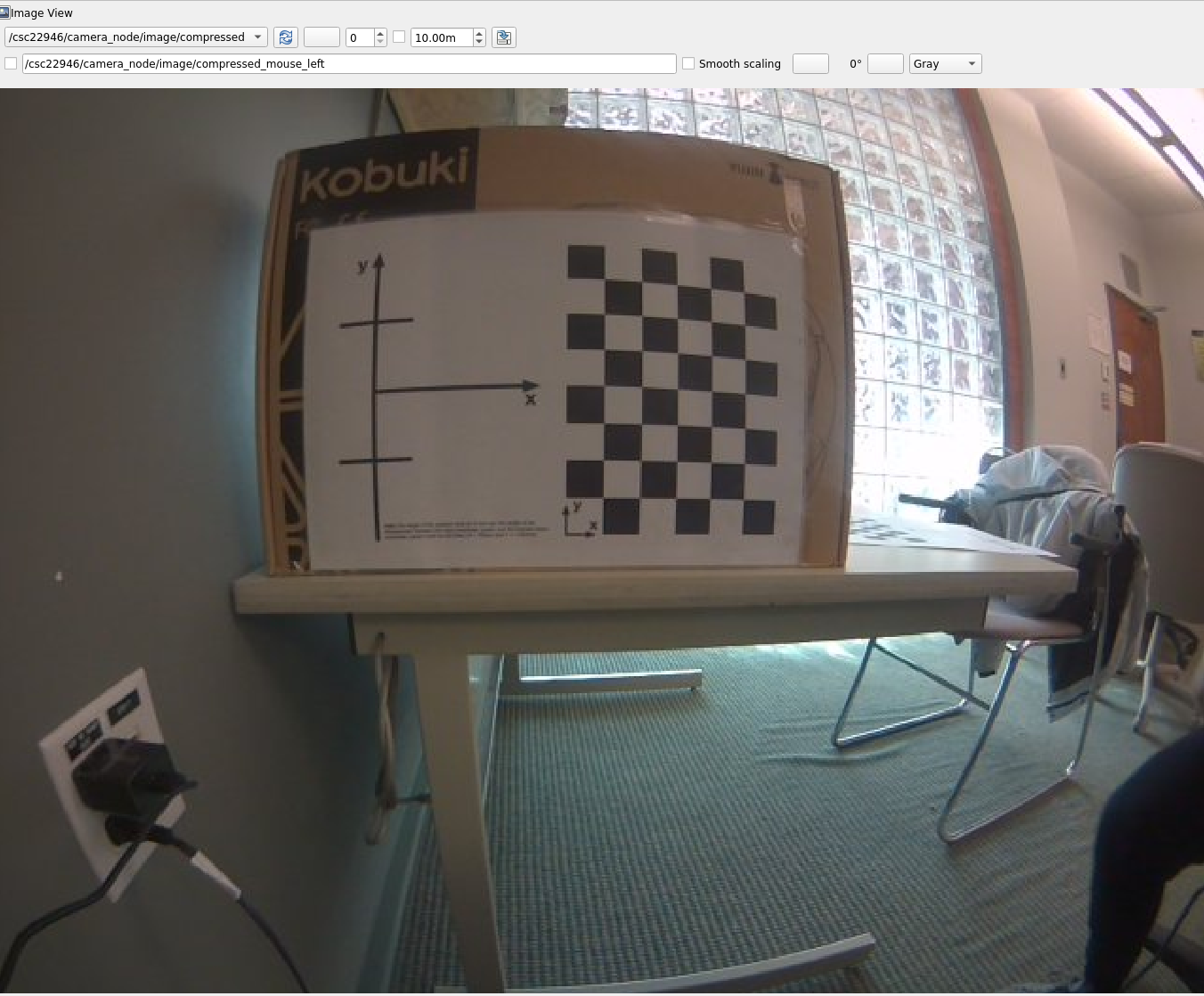
Distorted

maes — Figure 1: distorted image. Simply a raw image gotten from the bot.

Undistorted

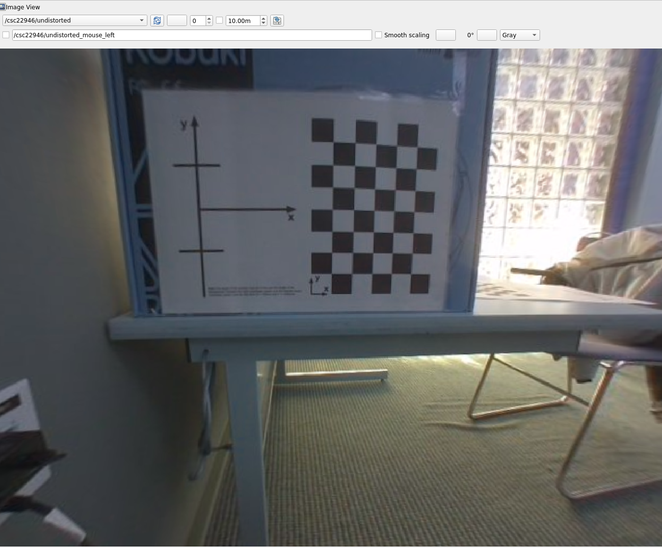
To undistort the image, we grab the K and D matrices from the camera_info topic. K is the intrinsic parameter matrices and D is the distortion coefficient matrices. We use CV2’s undistort method to do the job. Code here.

Image recognition

We used the code from this tutorial by GeeksforGeeks.

We first find the lower and higher hsv value for color of interest. We did that manually using a color picker.
hsvFrame = cv2.cvtColor(cv2_img, cv2.COLOR_BGR2HSV) convert cv2_img to HSV tensor.
we compute mask by activating all the pixels that are in range color_mask = cv2.inRange(hsvFrame, self.red_lower, self.red_upper).
Color mask when displayed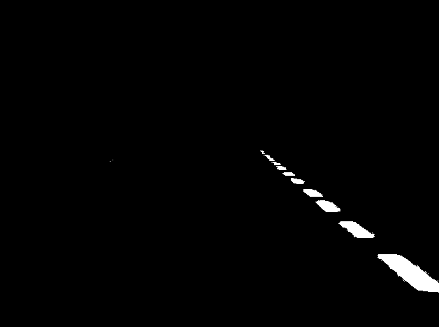
Then we dilate the mask to enlarge color object. color_mask = cv2.dilate(color_mask, kernel).
Color mask when displayed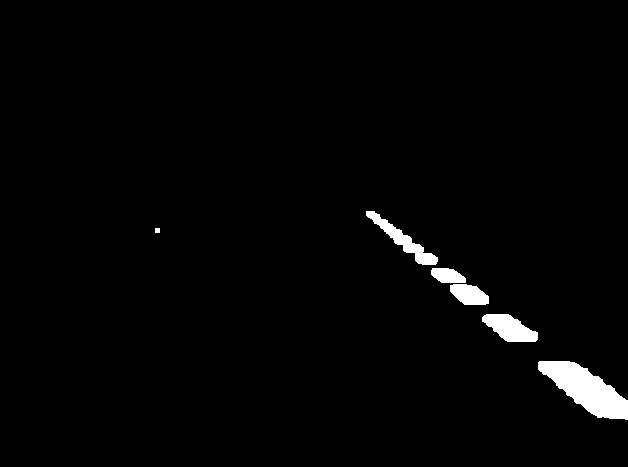

By Creating color_mask for each of the RED, BLUE, GREEN, WHITE, YELLOW, we can draw bouding box aroud them for visual purpose. colormask1

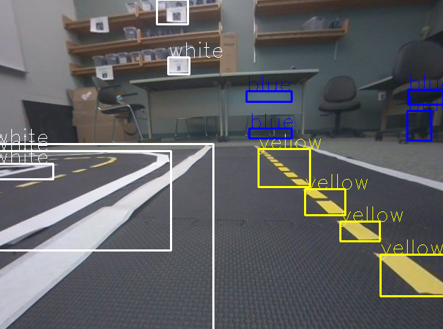
Colored Tape detection

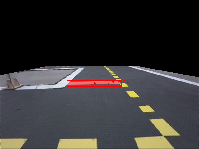
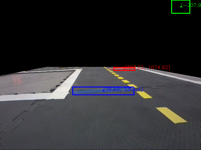
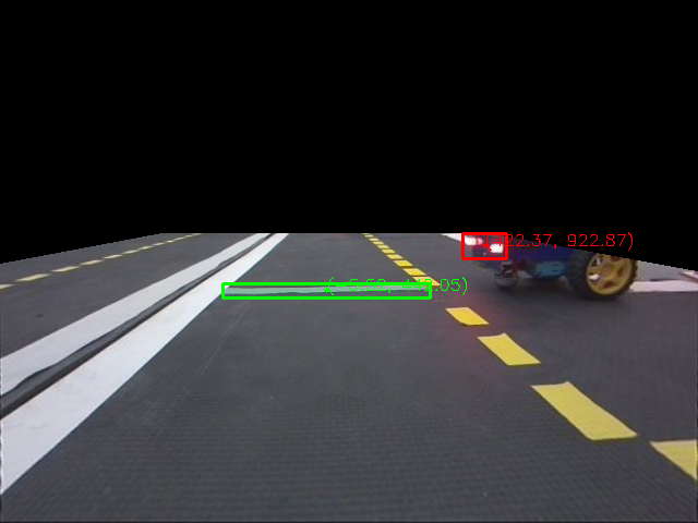
In these images, we mask out the background to avoid detecting background objects. We had to tune the V number in HSV since tape colors in different rooms were darker due to light conditions. Not sure what else to say to explain these images.

Tuning of HSV value

Selecting the hue ranges for each colors were simple. We went to color picker website like this one. Only thing to keep in mind was that cv2’s hue range is 0 to 170, while color picker hue ranges were 0 to 255, so we had to scale the range.

Projection using homography

We need a way to know the distance between the bot and the real object that it sees with the camera. Therefore, we have to somehow project the image onto a real world coordinate system.

Get homography matrix

A homography matrix maps between coordinate system in the image to the coordinate system in the real world. The inverse of this matrix will make an inverse map that maps the real world coordinate system back onto image coordinates. Having a projection to ground is important to have an estimate of the distance between the real object and the bot.

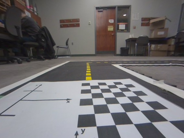
We get the mapping by grabbing real world coordinates of the calibration checkerboard, in militers, and grabbing the corresponding pixel coordinates on the image. Aforementioned, each tile is 31mm x 31mm, and we get the four corners of the checkerboard. Therefore, we define the ground points on the calibration checkerboard as [0, 0], [186, 0], [0, 186], [186, 186]. We then get coordinates of these four corners in the image to be [284, 285], [443, 285], [273, 380], [584, 380].

We applied cv2.findhomography(img_points, checkerboard_points) to get the self.homography_to_ground matrix that can maps between these two coordinate systems.

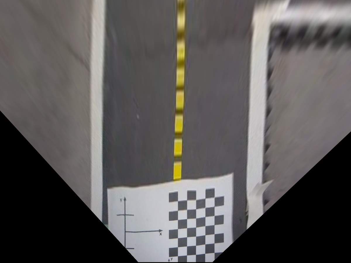
And voila. We can project any pixel point to the real checkerboard coordinate system using cv2.warpPerspective() The projected image based on the homography matrix looks like this. Thus, the difference in pixel points in the projected image is equivalent to distance in the actual object, in milimeters.

Stopping before colored tapes

To integrate computer vision, LED control, and wheel movement nodes, we used ROS services. The odometry and wheel movement nodes from lab 2 is in the Move node. This node acts as a server that provides the services {drive_straight/rotate/drive_arc/pause/drive_turn}_request. The node color_based_movement is the only client to use these services for the stopping tasks below. The LED control does not have its own node. It simply exist inside color_based_movement node. Lastly, we have the node camera_detection node that detects colored_object, do projections, and uploads the coordinates of the nearest colored objects onto {vehicle_name}/color_coords topic.

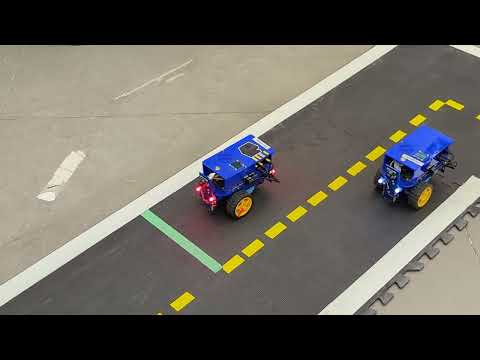
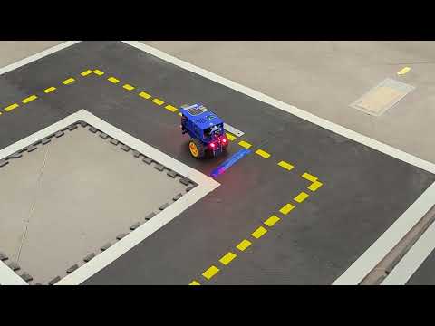
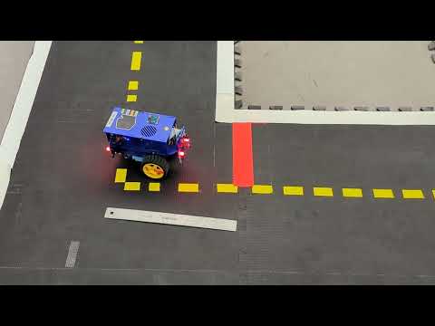
We have the node color_based_movement.py to do the stopping tasks. In this node, we subscribe to {vehicle_name}/color_coords topic to get the the coordinate of nearest color object at any time. The publisher of this node is camera_detection node. In the movement() function, we have a loop to stop when the distance to these color tapes are close enough.

After the bot stops in front of the colored line, it executes next actions accordingly. For example, if it stops in front of a red line, it will publish to LEDcontrol node accordingly and calls the drive_Straight service with the json parameter

{ "meters": meters, "speed": speed, "leds": leds}.

We can improve the modularity of this integration by having a separate node for LED controls. However, it will incur more latencies with additional service calls to the LED node. To optimize for delays with service calls to the move node, we simply stopped using the move node. Instead, all the movements are done using Twist2dStamped message. `😀

To answer part one Q6 b) iv), the higher camera frequency does not affect the integration. The rate of camera processing is determined by the main control loop in camera_detection node.

Part two: Controllers

Prerequisite: Error Computation

The controller requires us to calculate an error value for it to minimize. These steps are done in camera_detection node under the function perform_camera_detection.

project and draw line of best fit

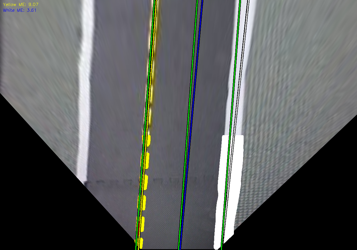
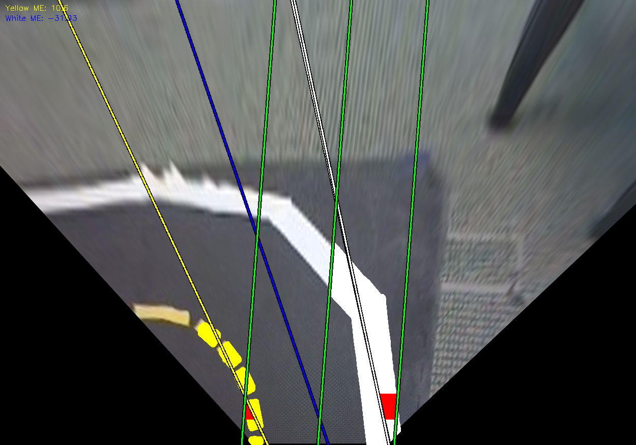
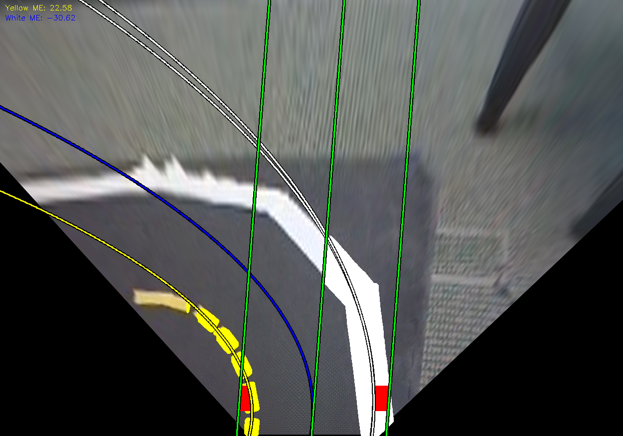
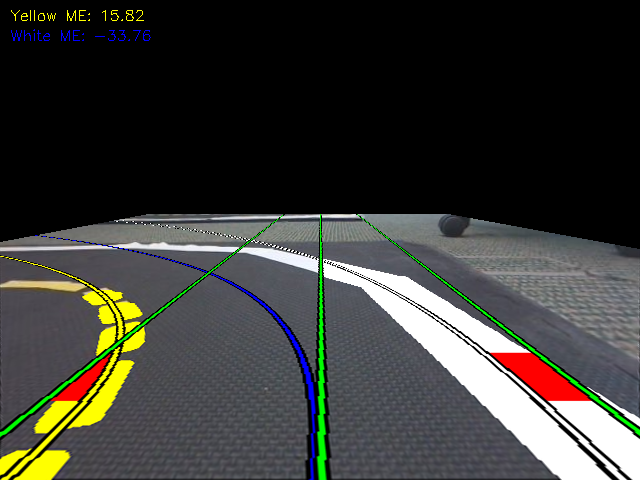
First we project image onto the checkerboard coordinate system. Then, we pre-define a target tangent lines on both side (the line in green). This green tangent line represents the camera orientation with respect to white/yellow lines in order to follow lane.

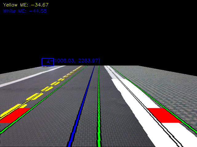
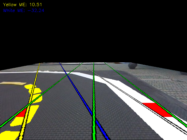
We detect all the yellow and white pixels in an image and compute the degree=1 line of best fit for yellow and white detected lines. This returns the tangent line coefficient.

We compute 2 errors. An error between the detected yellow/white lines and the target tangent lines on each side. We publish these 2 errors as {yellow: yellow_error, white: white_error} into {vehicle_name}/maes topic for the controller node to use.

Visualize:

These images are projected back onto the old coordinate system for visualization purposes.

Straight Line with controllers

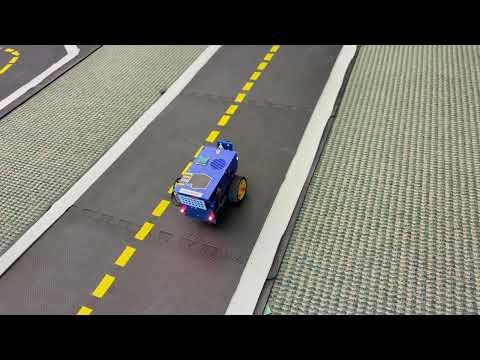
P contrller — P controller straight line. Click me

We tuned P values in the range [-0.0234, -0.03125], we settled for -0.0234. The straight line task is already good with just P

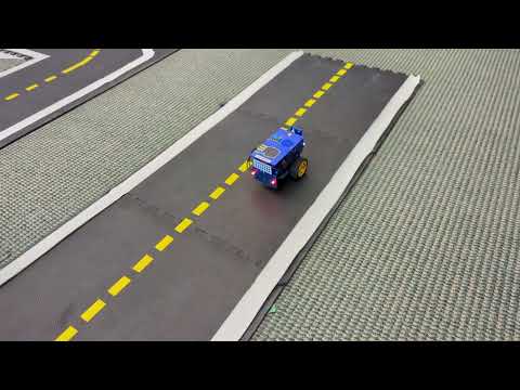
PD contrller — PD controller straight line. Click me

Just like the theory, it helped with dampening the oscillation at the end.

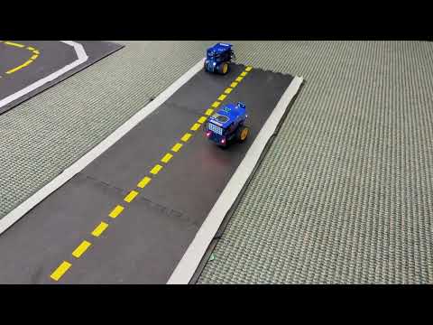
PID contrller — PID controller straight line. Click me

The bot was more unstable with the integral term. We suspect that the bot never reached the steady state where the cummulative errors are small. Therefore the integral term was big and it contributed big toward the final controller output. The bot did well without integral term, so adding it just increased the output angle by a factor of integral term, causing more oscillation.

We have a controller node. In this node, we subscribe to {vehicle_name}/maes, a the error values for the controller to minimize. Aforementioned, the publisher of this topic is the camera_detection node.

In the controller node, we have a loop that outputs a steering angle value that we clamp between \([-2\pi, 2\pi]\). This performs straight line task pretty easily.

Pros, cons, differences between controllers

P controller

Pros:
-Only variable is the proportional gain \(K_p\). It adds immediate feedback to the errors. Simple to understand the behavior Cons:
-Sensitive to small gain changes. The bot overshoots during correction, causing high angles. Tune:
-Through trial and error, we tried values between -0.3 to 0. -Since the contribution of the P term toward steering angle is \(K_p \cdot error\), we want the product to be negative if the error is positive (bot need to steer left, a negative angle) and vice versa.

PD controller

Pros:
-Reduces oscillations and improves stability by taking into account of the rate of change term (derivative). Cons:
-Caused overshooting output when the error term increased rapidly when bots were turning. Tuning:
-The contribution of the D term toward steering angle is \(K_d \cdot derivative\). So we want the sign of this product to be same as of the P term. Therefore, we se the value of \(K_p\) term to be negative to oppose the rate of error change, dampening the oscillation.

PID controller

Pros:
-In theory, eliminates steady-state error.
Cons:
-Hard to tune since we have to tune the previous 2 terms.
Tuning:
-We haven’t tune the I term yet.

Part 3: Lane Following

Challenges

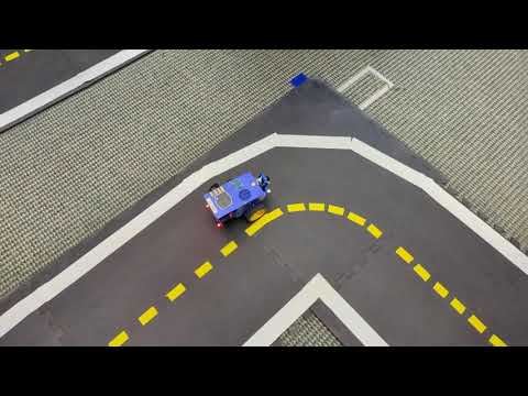
The approach to compute errors described in lane following did not work well in the circle track. The reason is because the latency due from error computation is high despite building and running the container on the bot. When the bot approach the curve, the error changed rapidly. This requires the error value to be up-to-date. Otherwise, the bot will turn too much or turn too little on the curve, and this is exactly what happened. Another reason why it overshoots is that the Twisted2DStamp message changes the wheel velocity to accomodate big change in angles, exercerbating overshoot during turns with latencies.

Solution

We implemented a simpler version of error computation for the controller in perform_simple_camera_detection(). We only follow the outer white line.

In that function, we crop the camera image to bottom left or bottom right depending on where the white line is.

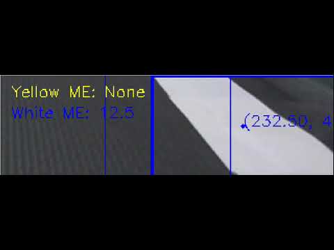
Then we find the center point of the detected white-lane contour, and we get the midpoint of it. The error is the difference between the center of the contour and and some offset from the left of the camera (it acts as a center point). Look here for the detail.

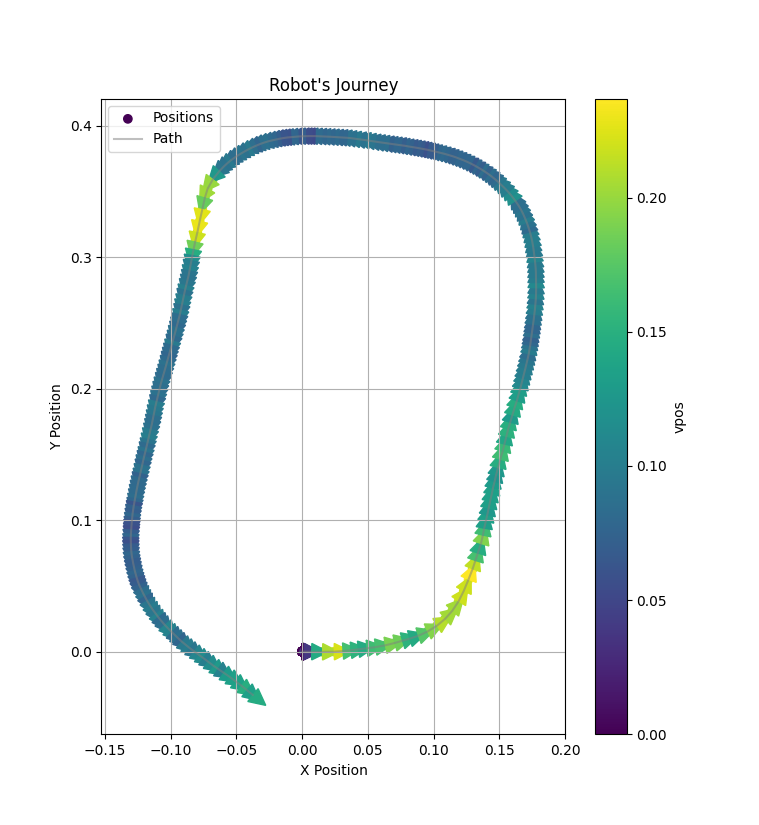
Watch the video — Video of live error detection. Click me

Then Voila! We can follow the circle using same \(K_p, K_d, K_i\) as the straight line task.

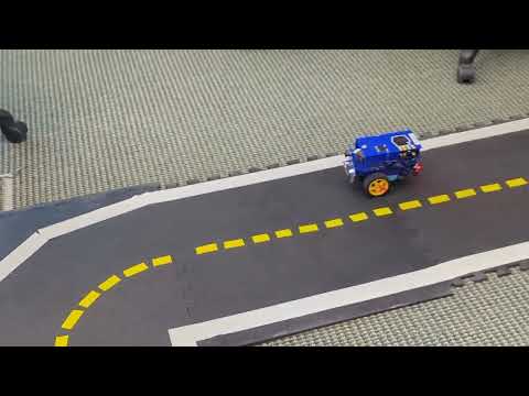
Exactly the same code as the straight line task with the same PID parameters. We published the Twisted2DStamped msg to the wheel_cmd with constant velocity of 0.23 and the turn angle from the controller. The container is built and ran on the bot to reduce the network latency.