CMPUT 503 Lab 4 report

Team member: Truong-Giang Pham, Nicolas Ong, Martin Mclaren

1. AprilTag Detection

AprilTags are a visual fiducial system, meant for use in computer vision, augmented reality, robotics, and embedded systems applications [1]. Each tag serves as a fixed reference point, and can be accurately and efficiently detected in an image using the provided software. In particular, AprilTags are designed for localization in a scene, allowing us to obtain a highly accurate estimate of its position (x, y, z coordinates) and orientation with respect to our camera (especially useful for the bonus objective in this exercise). For our purposes, however, it is sufficient to just detect a tag in a scene and obtain its corresponding ID. We use the dt-apriltags library for tag detection in our code, a Duckietown wrapper of the original apriltag library created by AprilRobotics.

Image Preprocessing for Tag Detection

As is standard with virtually all computer vision tasks, it is first necessary to perform image preprocessing. By eliminating unnecessary features within (and variations across) data samples, preprocessing helps to reduce the gap between the expected format of the data our algorithms are designed to work with, and the actual data they receive as input from our system, ensuring they function correctly. For the task of AprilTag detection, our preprocessing steps ensure the relevant features of the tag are made salient (black and white squares), and other features are reduced or eliminated. The steps we applied are as follows:

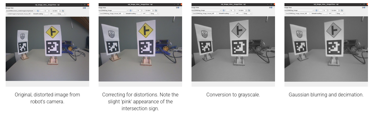
We first correct distortions introduced from our Duckiebot’s camera with cv2.undistort(), using the homography matrix we obtain from performing camera calibration. For the purposes of AprilTag detection, this ensures that the edges of the tag and each data ‘cell’ are all straight, which is critical for the detector to work correctly.
Next, the image data is converted to grayscale using OpenCV’s cv2.cvtColor() and the COLOR_BGR2GRAY colour space. This step is necessary as sources of coloured light (or reflections of white light off of coloured surfaces in the environment) can change the appearance of especially the white cells in each tag, possibly interfering with detection. This is illustrated in images 1 and 2 below, where the closer intersection sign has a warmer hue when compared to the University of Alberta sign due to light from our robot’s LEDs.
We blur the image using cv2.cvtColor(). This helps to reduce the effect of any noise in the image data and makes the relevant features of the tag more salient location, i.e. size of each cell’s edge with respect to the other cells’, as well as the border of the entire tag. While blurring will limit the detector’s ability to detect tags far in the distance, as individual cells will appear blurred together, this is not a concern for the distance scales we are working with in this project.
Lastly, the image is decimated (i.e. resolution is reduced) using cv2.resize(). This is not strictly necessary to improve tag detection performance, but instead reduces the computational overhead required for detection, thus freeing up resources for use by other programs in our system (namely: navigation).

Detecting AprilTags

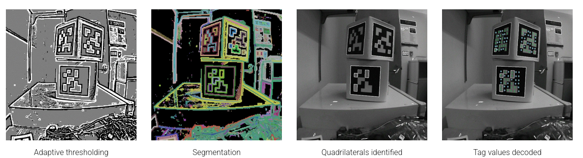
The AprilTag detection algorithm works as follows (images and details sourced from [2]):

Adaptive thresholding is first applied to the image to differentiates light pixels from dark ones.
Image segmentation is used to identify and isolate continuous regions of either only light or only dark pixels (i.e. the cells in the tag). Segmented regions that are too small are considered to not be part of any tag, and are ignored.
Quadrilaterals are then fit to the previously obtained segments. Relatively large quadrilaterals that contain many smaller ones are considered good candidates for the borders of a tag. The geometry of this candidate is used to obtain the center of the tag.
With the outline of a tag identified, individual cells contained within this outline are identified, and decoded as either 0 or 1, depending on the intensity of each cell. These values are used to identify the ID of the tag.

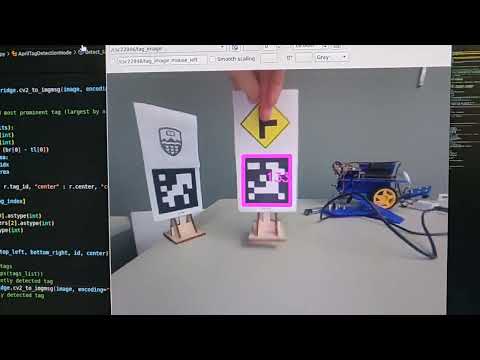
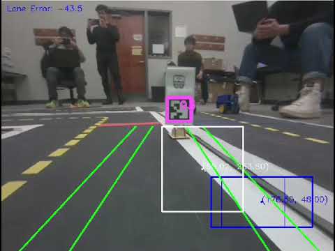
This algorithm returns the corners, centers, and IDs of all tags detected in an image (as illustrated in the above photos). For this exercise, tags are used to instruct our robot on how to navigate through its environment, such as which direction to turn. Our system therefore needs to be able to discriminate between multiple tags, and identify which is immediately relevant and which can be ignored. We do this by obtaining an estimate of the area of each tag in the image plane using their corner coordinates as provided by the detector. This acts as a proxy for the tag’s proximity to our robot, under the assumption that all tags are oriented similarly with respect to the camera. With this, we can choose to only register the closest (i.e. largest) detected tag. Our tag detection, and this behavior in particular, is demonstrated in the below video. Note also that this approach can easily be adapted to ignore any tags that are beyond a certain distance from our robot.

Our robot has only a limited number of computational resources available, and these must be distributed such that each running process receives all and only those resources required for it to perform its function. The refresh rate at which each process is run at is a significant contributor to its total cost, and so an important optimization strategy is setting the lowest rate possible. For AprilTag detection, we use a lower rate (3Hz) for the main detection loop compared to other processes on our system. Unlike tasks such as lane-following, where errors can accumulate quickly resulting in large deviations off course, there is little moment-to-moment change involved with detecting AprilTags. Detected AprilTags have a constant value, and even when the detection is lost, this value is stored in our system’s memory. Using a lower detection rate frees up resources for other processes on our system, while not hindering detection performance.

This low rate is also suitable for other situations where, say, AprilTags serve the function of traffic lights. With an even lower rate (say, 1Hz), the worst-case result is a ~1 second delay between light change and response by our robot. Even in real-world autonomous driving, which is conducted at higher speeds and with greater stakes, this delay would be more than acceptable, and indeed falls into the range of typical human performance.

We program our detection loop to act as as interrupt for our robot’s regular behavior (i.e. continue doing previous command until a tag is detected, than change behavior). As such, a lower detection rate slightly increases the ‘reaction time’ of our robot, which can result in longer stopping distances or stop times at stop lines, though not to a significant enough degree that it impacts our robot’s ability to navigate through the track, such as driving through or turning in intersections. One nuisance caused by adjusting the rate, however, is the impact it has on the duration of wait() calls in our code, requiring us to tweak its values to get our robot to stop for the desired amount of time after seeing a tag or stop line.

Lane following with AprilTags (including bonus)

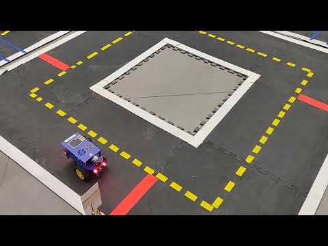
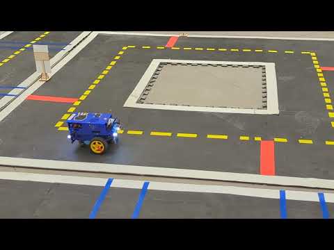
We use our lane following routine from Exercise 3 (described here) in conjunction with AprilTag and colour detection to perform the loop shown in the videos below. Here, our robot navigates a square track (that features three AprilTags that function as road signs), stopping at each red line. The duration of each stop is determined by the last detected tag. When a tag is detected, our robot also sets its LEDs to reflect this.

Stop sign: duration of stops = 3 seconds, LED colour: red
Intersection sign: duration of stops = 2 seconds, LED colour: blue
University of Alberta sign: duration of stops = 1 second, LED colour: green
Default (no sign): duration of stops = 0.5 seconds, LED colour: white

A note on the above procedure: as a tag is detected in the distance, our Duckiebot changes its LED colours as above. As the robot comes within a certain distance of the red stop line, it stops with LEDs still set (at this point, it has lost detection of the tag). After stopping for the above duration, the LEDs are set to their default and the robot continues on its path.

Our lane following algorithm struggles to navigate around sharp corners. To overcome this, we implement the following fixed maneuver: when a white lane marker is detected directly in front of the robot (and within a certain distance threshold), the robot stops and performs a rotation (tracking how many degrees it has rotated) until the white contour is detected to the right, after which normal lane following can resume. We can see this behavior demonstrated in the videos below, where our Duckiebot completes two full laps of the track, detecting all tags and responding accordingly.

2. PeDuckstrian Crosswalks

To detect crosswalks, we use the same colour detection technique we developed in the previous exercise. We first convert the RGB pixel values from the Duckiebot’s camera to HSV values, and then generate a mask for any colours falling within a thresholded range (see below), that we tune for best performance given the environmental conditions in the lab (lighting, specific colour of tape used for road markers, etc.).

HSV value range for blue detection:

self.blue_lower = np.array([110, 80, 120], np.uint8)

self.blue_upper = np.array([130, 255, 255], np.uint8)

Once a contour of the appropriate colour is detected, we can obtain an estimate of its distance from our robot and, once near enough to our robot, send an instruction for it to stop. We use the distance of the closest blue line to gauge when to perform the stop. If no pedestrians are detected in the crosswalk, the robot resumes its forward path after 1 second. To ensure that it doesn’t immediately stop again at the second line in the crosswalk (i.e. right in the middle of the crossing), we set a small cool down on the stopping behavior, during which the robot will continue with its previous trajectory. As above, we use our lane following algorithm with PID control to ensure our robot stays centered on the road. Waiting for peDuckstrians

As with lane feature detection, we again make use of colour masking to perform pedestrian detection. While stopped at a crosswalk, a second colour mask is generated for all pixels that fall into the orange range listed below. If any pixels are activated in the mask, our robot remains stationary at the crosswalk until they disappear (i.e. until the pedestrians have finished crossing the street).

HSV value range for orange detection:

self.orange_lower = np.array([30/2, 50*2.55, 30*2.55], np.uint8)

self.orange_higher = np.array([36/2, 100*2.55, 100*2.55], np.uint8)

As the colour of the pedestrians closely matches that of the yellow lane dividers, much more effort was spent finding and tuning a range of values that would detect the former but exclude the latter. For added robustness, we additionally check to make sure that the area of the detected contours was above a certain threshold, which we set to roughly correspond to the expected size of the ducks at the distance our robot stops from the crosswalk. This further ensured lane dividers would not be excluded during this masking, as well as any errant small groups of pixels that may be detected in the background. With these adjustments, our robot reliably detects and waits for pedestrians to clear the road before proceeding.

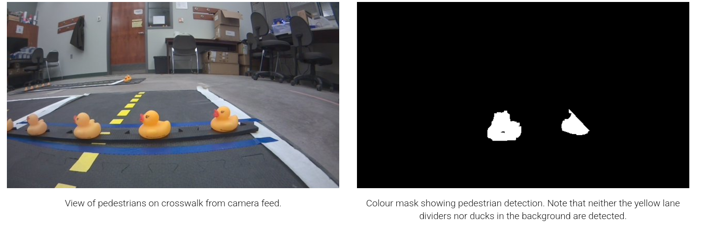
While sufficient for this exercise, this technique would fail under variable lighting conditions, which could change the perceived colour of the pedestrians sufficiently that they are no longer detected by our mask. Even under constant lighting conditions matching those in the lab, the colour of the pedestrians can vary drastically with factors like distance and orientation, posing potentially more problems for our detection.

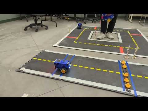
The video below shows our Duckiebot safely navigating crosswalks both with and without pedestrians, traveling straight along the path thanks to our lane following implementation. At the first crosswalk, our robot comes to a stop for roughly 1 second before proceeding straight through. At the second, our robot continues to wait until the pedestrians have been cleared from the scene. In rewatching this video, we note that the robot stops with some distance away from the blue crosswalks. For our final exercise, additional tuning of our stopping criteria will be performed to reduce this, such that our robot stops just before the crosswalk.

Detecting other Duckiebots

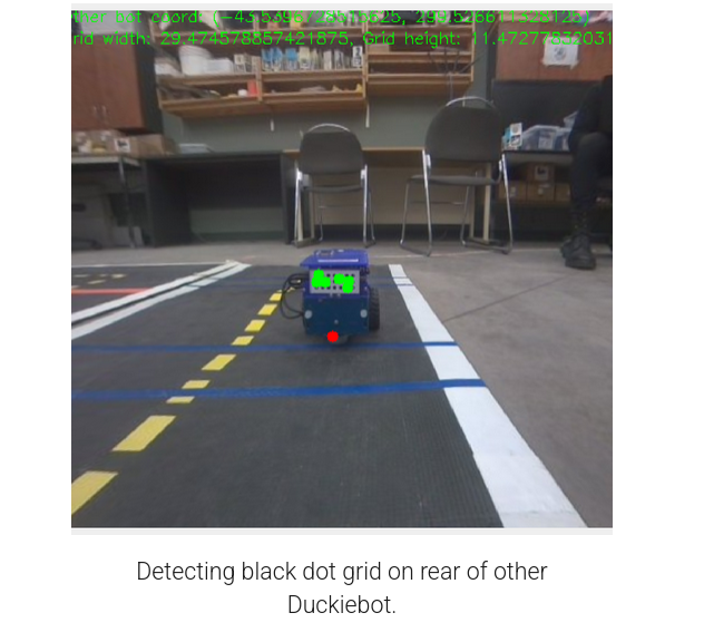
We wanted to implement a non-colour based detection technique for identifying other Duckiebots, as we noted that the colour of the robots is very similar to that of the blue tape used for crosswalks. We were particularly unsure if this conflict would cause problems for the final project, and so looked to use a geometry detection technique instead. We settled on attempting to detect the black circle grid found on the back of each Duckiebot using OpenCV’s SimpleBlobDetector(). The parameters passed to this function gave us a lot of flexibility in terms of specifying the kinds of shapes we wanted to detect, and we thought this approach showed a lot of promise for the task at hand.

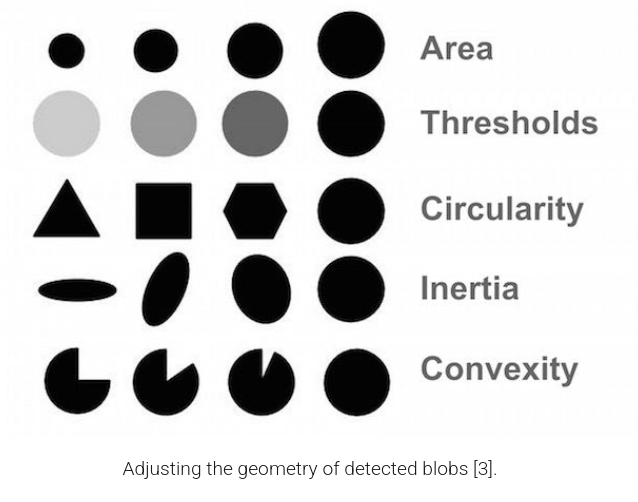
To aid in detection, we performed the same image preprocessing as before. After running the detector, we use our remove_outlier() function to first compute the middle detected point on the grid, and remove any outliers that fall outside a certain distance range from this point. We then visualize each detected point using green circles (shown in image below).

With these detected points, we then approximate the length and width of the backboard, and project a point straight down to the ground (drawn in red in the image below) that roughly corresponds to bottom of the Duckiebot. We lastly use our usual distance measuring technique to project this point to the world coordinate space, allowing us to get an estimate of its distance from our robot.

While sound in theory, this method proved to be extremely challenging to get working, and thus far remains the only task across all exercises we have been unable to solve within the time provided. In particular, this technique yielded highly inconsistent estimates for the distance of our robot from the broken-down Duckiebot. So, while our robot was often able to detect the presence of the other Duckiebot, it usually failed to stop in time, or stopped to early, which caused our collision avoidance maneuver (described below) to fail. These inconsistent estimates are due to the brittleness of the black dot grid detection. In particular, while our detector is always able to identify some collection of these dots, the number and specific set of dots would change on each run, being highly sensitive to even the smallest changes in lighting conditions. As such, the calculated dimensions of backboard changed on each run, yielding inconsistent distance estimates following projection.

In the challenges section below, we discuss how we might attempt Duckiebot detection using a simple colour mask in the future.

Bonus

a) Continuous AprilTag detection loop

References

[1] https://april.eecs.umich.edu/software/apriltag

[2] https://docs.wpilib.org/en/stable/docs/software/vision-processing/apriltag/apriltag-intro.html

[3] https://learnopencv.com/blob-detection-using-opencv-python-c/ 

Lab exercise guidelines